WindComfort-ML (VIP-SMUR Spring 2026)
WindComfort-ML is a collection of machine learning–based surrogate models for predicting ground-level wind flow in urban environments from building configurations.
These models approximate traditional Computational Fluid Dynamics (CFD) simulations in seconds, enabling rapid design iteration for architects, planners, and researchers. The system is designed to integrate with the Eddy3D plugin in Grasshopper, requiring little to no programming experience.
Overview
Traditional CFD simulations are computationally and time-intensive.
WindComfort-ML provides fast inference (seconds) and integration with Grasshopper / Eddy3D workflows for an accessible interface for simulation. We include multiple models for testing and development.
Models
Each architecture has a folder under models/. Some folders contain local model code, while externally maintained implementations are linked or included as Git submodules. Find the model weights below. Additional details (e.g., training pipelines, datasets) may be linked to external repositories where applicable.
| Architecture | External Repo | Model Weights | Notes |
|---|---|---|---|
| Conditional Transformer | Link | TBD | |
| Fourier Neural Operator | Link | TBD | |
| Generative Adversarial Network | Link | TBD | |
| Latent Diffusion | Submodule / External repo | Link | Included as a Git submodule. |
| Graph Neural Network | Submodule / External repo | TBD |
Specific instructions for inference, evaluation, and expected data formats can be found in the README of each model folder or in more detail in the linked repos.
📂 Repository Structure
WindComfort-ML/
├── README.md
├── .gitmodules
└── models/
    ├── conditional_transformer/
    │   └── README.md
    ├── fno/
    │   └── README.md
    ├── gnn/                 # Git submodule: NishanthG05/GNN-RANS-Flow
    ├── ldm/                 # Git submodule: alec-y-cheng/latent-diffusion
    └── pix2pix/
        └── README.md
To clone this repository with the Latent Diffusion submodule included:
If the repository was already cloned without submodules:
Dataset Specification
As many of our models were based off general image generation (which operates on 3-channel RGB images), this pipeline has been modified to map 8-channel physical geometry inputs mapping to 1-channel wind deficit predictions.
The model expects inputs and outputs where each channel is normalized around [-1, 1] for the generator.
📥 1. Input Tensor (X)
Shape: [8, Height, Width]
The input consists of 8 channels representing physical geometry and wind conditions.
| Idx | Name | Description | Normalization | Range (Approx) |
|---|---|---|---|---|
| 0 | SDF* | Signed Distance Field (distance to nearest wall) | / 200.0 | 0.0 – 1.0 |
| 1 | Bldg_height | Height of the building at this pixel | / 50.0 | 0.0 – 1.0 |
| 2 | Z_relative | Height slice of the simulation (Z coordinate) | / 10.0 | 0.0 – 1.0 |
| 3 | U_over_Uref | Background wind ratio (inlet profile) | * 2.0 | 0.2 – 2.0 |
| 4 | X_local | X distance from building center | / 500.0 | -1.0 – 1.0 |
| 5 | Y_local | Y distance from building center | / 500.0 | -1.0 – 1.0 |
| 6 | dir_sin | Sine of wind direction | None | -1.0 – 1.0 |
| 7 | dir_cos | Cosine of wind direction | None | -1.0 – 1.0 |
*In models trained on directionally integrated distance (DID) function, there are 7 additional input channels, each channel representing DID values at each coordinate for each of the 8 input directions.
2. Target Tensor (Y)
Shape: [1, Height, Width]
The model predicts a single scalar value representing the wake deficit:
Target_Delta_U = (Mag_U - U_ref) / U_ref
Interpretation
0.0→ No change (wind speed =U_ref)-0.5→ 50% drop in speed (strong wake)-1.0→ Stagnation (wind speed = 0)
Reconstruction Formula
To recover actual wind magnitude:
Mag_U = (Prediction * U_ref) + U_ref
Methodology & Evaluation
Design Approach and Evaluation Strategy
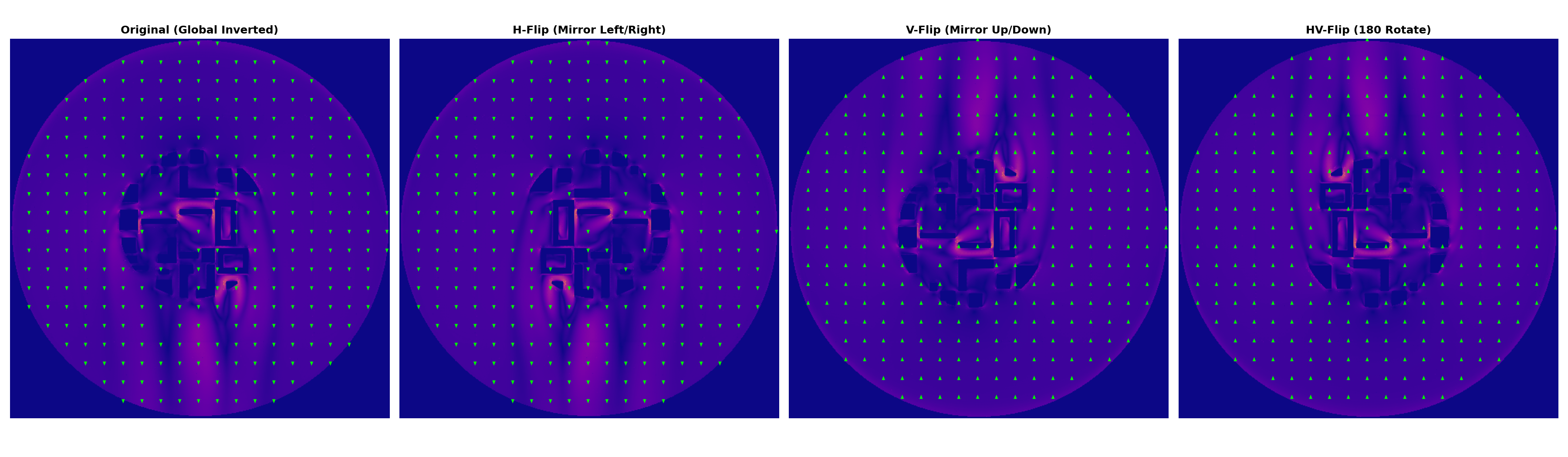
All models were initially evaluated using a geometric proxy representation of the flow field based on a [Signed Distance Function (SDF) / Directionally Integrated Distance (DID)] formulation.
Rather than directly predicting full CFD solutions at the outset, this approach allowed us to:
- Establish a consistent and computationally efficient evaluation baseline
- Compare model behavior on spatial structure before full physical rollout
- Reduce noise from simulation-specific artifacts
Our methodology builds on top of existing state-of-the-art (SOTA) architectures by incorporating physics-informed loss functions.
We begin with baseline models (e.g., CNNs, UNets, ViTs, etc.). augment training with additional constraints that encourage physical consistency, often loss functions that enforce physics based on Navier-Stokes equations. We also infer based on specialized metrics that push our models away from pure image generation (which prioritizes RMSE pixel loss), and towards physically-informed targets (like gradient correlation).
Evaluation Metrics
Models are evaluated and inferred against ground-truth CFD simulations using:
- Root Mean Squared Error (RMSE)
- Mean Absolute Error (MAE)
- Mean Absolute Percetange Error (MAPE)
- Structural similarity (SSIM)
- R-Squared (R2)
- Gradient Correlation (GradCorr)
- Inference time
Sample Inference
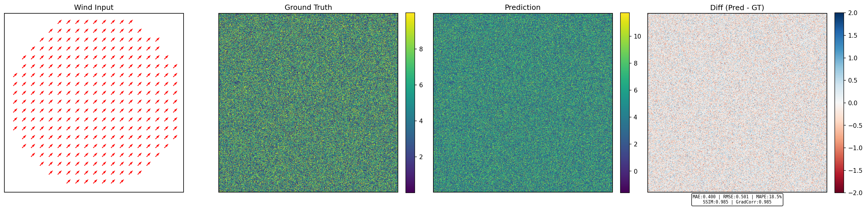
Repositories have their own tailored inference scripts that test models on the above evaluation metrics.
Model Evaluation
Each architecture's best model performance is displayed below:
| Model | RMSE ↓ | MAE ↓ | MAPE (%) ↓ | SSIM ↑ | R² ↑ | GradCorr ↑ | Inference Time (s) ↓ |
|---|---|---|---|---|---|---|---|
| Conditional Transformer | TBD | TBD | TBD | TBD | TBD | TBD | TBD |
| FNO | TBD | TBD | TBD | TBD | TBD | TBD | TBD |
| Pix2Pix | TBD | TBD | TBD | TBD | TBD | TBD | TBD |
| LDM | 0.062 | 0.034 | NA | 0.911 | 0.317 | 0.513 | 0.7 |
| GNN | TBD | TBD | TBD | TBD | TBD | TBD | TBD |
Presentation