MPONC — Modeling Processes of Neighborhood Change
An agent-based simulation framework for modeling residential relocation dynamics across census tracts in metro Atlanta (Fulton & DeKalb counties). MPONC simulates how households choose where to live based on affordability, amenity access, community fit, and proximity to the Atlanta BeltLine, then calibrates model parameters against observed Census data. The framework supports three distinct relocation models—No Regret Dynamics (Legacy), Push/Pull, and Gravity—each offering a different mechanism for translating tract-level scores into relocation decisions.
Table of Contents
- Quick Start
- Project Structure
- Scoring System
- Relocation Models
- No Regret Dynamics (Legacy)
- Push/Pull Model
- Gravity Model
- Calibration
- Error Metric
- Configuration Reference
- Notes
- Team
Quick Start
Prerequisites
- Python 3.10.16
uv
Install
Run the simulation directly
Project Structure
mponc/
├── main.py                        # CLI entry point
├── run_calibration_suite.py       # Multi-year calibration runner
├── config/
│   ├── config.py                  # All simulation settings, hyperparameters, data endpoints
│   └── helper.py                  # Derived paths, directories, and convenience settings
├── src/
│   ├── calibration_logic/
│   │   ├── calibration.py         # PSO and RBFOpt calibration optimizers
│   │   ├── calibrate_all_years.py # Multi-year calibration orchestration
│   │   ├── error_metrics.py       # MAE, RMSE, MAPE, MSE, Max AE computation
│   │   └── sensitivity_analysis.py
│   ├── core/
│   │   ├── initializer.py         # Pipeline initialization and data loading
│   │   ├── processor.py           # Data processing and transformation
│   │   └── simulator.py           # High-level simulation coordinator
│   ├── initialization/
│   │   ├── gdf.py                 # GeoDataFrame construction from Census + OSM
│   │   └── scores/
│   │       ├── amenities.py       # OSM/Overpass amenity density computation
│   │       ├── beltline.py        # BeltLine proximity scoring
│   │       ├── community_scoring.py  # Simplified income-difference community score
│   │       └── morans_analysis.py    # Local Moran's I spatial autocorrelation
│   ├── simulation_logic/
│   │   ├── simulation.py          # Simulation manager and timestep loop
│   │   ├── City.py                # City state: tracts, agents, populations, scores
│   │   ├── Agent.py               # Agent representation
│   │   ├── cost_function.py       # Legacy, Push/Pull, and Gravity cost functions
│   │   ├── location_choice.py     # Discrete-choice relocation (Push/Pull & Gravity)
│   │   ├── convergence.py         # Regret-based convergence detection
│   │   ├── counterfactuals.py     # Counterfactual regret computation
│   │   ├── feature_transforms.py  # Log-amenity and feature normalization
│   │   ├── error_metric_plot.py   # Calibration error progression plotting
│   │   └── sobol_analysis.py      # Sobol sensitivity analysis
│   ├── utils/                     # File naming, persistence, caching utilities
│   └── visualization/             # Choropleth GIFs, convergence plots, cost components
├── coefficients/                  # Calibrated coefficient sets (per model × year)
├── data/                          # Cached Census, OSM, and GeoDataFrame data
├── figures/                       # Generated visualizations
├── pyproject.toml
└── uv.lock
Scoring System
All three relocation models share a common set of per-tract scores computed from Census and OpenStreetMap data. These scores are recomputed at every simulation timestep based on the current agent positions and are normalized to [0, 1] to represent the desirability (or stress) of a census tract along different dimensions.
Affordability Score
A binary indicator of whether a household can afford a tract. An agent's income is compared to the tract's median income — if the agent can afford the tract, the score is 1.0; otherwise it is 0.0.
Upkeep Score
A capacity utilization measure for each tract, defined as the ratio of the current simulated population to the tract's housing capacity (ρ):
Upkeep of 1.0 means a tract is at full capacity; lower values indicate available housing stock. The legacy model treats upkeep as a multiplier on tract quality; the push/pull and gravity models use it as a penalty signal.
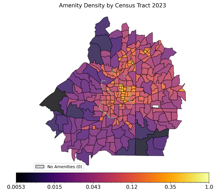
Amenity Density Score
Derived from OpenStreetMap (Overpass API) point-of-interest queries. Amenity categories include restaurants, schools, grocery stores, transit stops, and commercial land use. Raw amenity counts per tract are transformed via a log-normalization that compresses the heavy-tailed density distribution:
This produces a score in [0, 1] that ensures differences between moderately and highly amenitized tracts remain meaningful, while tracts with zero amenities are clipped to the minimum positive value.
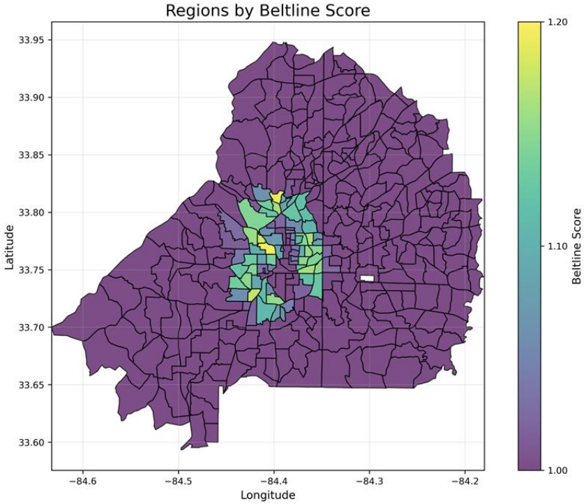
BeltLine Proximity Score
Measures each tract's distance to the Atlanta BeltLine trail network. Tracts closer to the BeltLine receive higher scores, decaying linearly out to a calibrated outer radius beyond which all tracts receive a baseline score. The inner/outer radii and the maximum BeltLine score are calibrated parameters.
Community Score
Measures how well an agent "fits" the socioeconomic composition of a tract. Two approaches are available:
- Simplified (default): Computes the absolute difference between the agent's income and the tract's simulated average income, normalized by the global income range and subtracted from 1.0. Agents in tracts with similar incomes receive scores close to
1.0. - Local Moran's I: A spatial autocorrelation statistic that captures income clustering patterns using expanded county data (13 counties surrounding Fulton/DeKalb). More computationally expensive and requires an additional calibratable distance-decay parameter (γ), but is theoretically grounded in spatial econometrics.
The simplified approach is used by default across all models, as it is faster to compute and requires fewer calibration parameters. Furthermore, additional testing and verification may be required to ensure the Local Moran's I feature works as intended.
Relocation Models
MPONC implements three alternative models for how agents decide where to relocate. Each model uses the shared scoring system above but combines the scores differently to produce relocation probabilities.
1. No Regret Dynamics (Legacy)
The original approach based on multiplicative weights update (MWU), a no-regret learning algorithm from online convex optimization.
How it works:
- Each agent maintains a probability distribution over all census tracts (the "action space").
- At each timestep, agents sample a tract from their distribution and observe the resulting cost.
- Costs are computed using the legacy cost function: where
attractiveness = (1 − λ) × amenity_score + λ × community_score. The parameterλ(lambda) controls the relative weight between amenity access and community fit, andMis an exponent controlling the sensitivity of cost to attractiveness. - Agent distributions are updated via MWU: Actions with higher costs receive exponentially lower weight, and the distribution is renormalized.
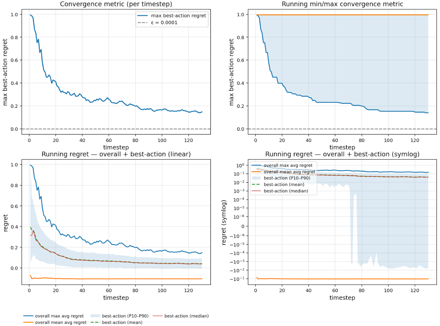
- Convergence is detected by monitoring the maximum per-agent "best-action regret"—the difference between the agent's realized average cost and the cost of the best single action in hindsight. When this metric falls below a threshold
εfor a specified number of consecutive timesteps, the simulation terminates early.
Strengths: - Theoretically well-founded with provable convergence guarantees from game theory. - Produces equilibrium distributions that represent stable population configurations.
Limitations: - Performs well in theoretical and synthetic settings but does not reproduce empirical Census income distributions well in case-study evaluations (RMSE ≈ 41,185 on the 2023 benchmark — substantially higher than the other two models). - The MWU learning dynamic does not naturally capture the asymmetry between staying and moving — all tracts are treated equally in the probability space regardless of how far they are from the agent's current location. - Convergence can require very large numbers of timesteps (T > 60,000), making calibration expensive.
2. Push/Pull Model
A discrete-choice relocation model that explicitly separates origin-side "push" pressures from destination-side "pull" factors. At each timestep, every agent evaluates all candidate tracts and probabilistically selects one. This model replaces the MWU learning dynamic with a single-shot softmax choice at each timestep.
How it works:
- Push (origin) factors evaluate stressors in the agent's current tract:
stay_affordability— affordability stress (inverted sigmoid of affordability score).stay_crowding— current tract occupancy pressure.stay_displacement_affordability— interaction of BeltLine proximity with affordability stress (gentrification pressure proxy).-
stay_displacement_crowding— interaction of BeltLine proximity with crowding. -
Pull (destination) factors evaluate the attractiveness of each candidate tract:
dest_amenity— amenity access penalty (inverted saturating utility).dest_community— community fit penalty (income mismatch).dest_beltline— BeltLine proximity penalty.-
dest_crowding— projected occupancy if the agent were to move in. -
Friction factors penalize the act of moving itself:
move_origin_comfort— inverse of leave pressure; comfortable agents are penalized for moving.-
move_distance— normalized Euclidean distance between origin and destination centroids. -
Each factor has a calibrated weight. The total cost per agent-destination pair is a convex combination of all factors. Final relocation probabilities are computed via softmax over negative scaled costs, with a
choice_stay_bonusterm added to the agent's current tract to capture inertia.
Cost function:
cost(agent, dest) = Σ_f  w_f × penalty_f(agent, dest),    Σ w_f = 1
utility(agent, dest) = −β × cost(agent, dest) + bonus × 𝟙[dest = home]
P(agent → dest) = softmax(utility)
Where β = choice_cost_scale and bonus = choice_stay_bonus are calibrated parameters. A minimum probability floor is enforced to prevent degenerate distributions.
Features (10 calibrated weights):
| Feature | Type | Description |
|---|---|---|
stay_affordability | Push | Affordability stress at origin |
stay_crowding | Push | Capacity pressure at origin |
stay_displacement_affordability | Push | BeltLine × affordability stress |
stay_displacement_crowding | Push | BeltLine × crowding |
move_origin_comfort | Friction | Comfort penalty for leaving |
move_distance | Friction | Normalized travel distance |
dest_amenity | Pull | Amenity access at destination |
dest_community | Pull | Community fit at destination |
dest_beltline | Pull | BeltLine proximity at destination |
dest_crowding | Pull | Projected crowding at destination |
The push/pull model can also be paired with the no-regret movement framework (MOVEMENT_FRAMEWORK = "no_regret"), which uses the multiplicative weights update on the push/pull cost function instead of the legacy cost function.
3. Gravity Model
A two-stage gravity-style model inspired by spatial interaction theory. The model separates the relocation decision into (1) whether to move at all (binary) and (2) where to go (destination tract), analogous to classical gravity models in transportation and migration research.
How it works:
Stage 1 — Move or Stay: The probability that an agent leaves their current tract is determined by origin-side push signals. Conceptually, agents in affordable, uncrowded tracts are unlikely to move; agents under financial or displacement pressure are more likely to relocate.
move_signal = w_aff × stay_affordability + w_disp × stay_displacement_affordability
P(move) = σ(β × move_signal − bonus)
σ is the logistic sigmoid. Stage 2 — Destination Choice (conditional on moving): If an agent decides to move, destination probabilities are computed as a softmax over a gravity-style pull score:
dest_score(j) = w_a × amenity_j + w_c × community_fit_j + w_b × beltline_j + w_m × mass_j − w_d × distance_ij
P(dest = j | move) = softmax(β × dest_score)
Where mass_j = log(1 + population_j) / max(...) captures the agglomeration effect — tracts with larger existing populations exert more "gravitational pull."
Final probability: The final relocation probability for any tract combines the move probability from Stage 1 with the destination probability from Stage 2. Agents who decide not to move simply remain in their current tract.
Features (7 calibrated weights):
| Feature | Stage | Description |
|---|---|---|
move_affordability | Move signal | Affordability stress at origin |
move_displacement | Move signal | BeltLine displacement pressure at origin |
dest_amenity | Destination pull | Amenity access at destination |
dest_community | Destination pull | Community fit (income match) |
dest_beltline | Destination pull | BeltLine proximity |
dest_mass | Destination pull | Log-population agglomeration pull |
distance_friction | Destination pull | Distance decay (cost of moving) |
The gravity model currently achieves the best calibration fit among the three models (RMSE ≈ 2,326 on the 2023 benchmark), largely because the two-stage structure and explicit distance friction produce more geographically realistic relocation patterns.
Calibration
Approach
MPONC calibrates model parameters by minimizing the RMSE between simulated and observed tract-level median incomes. The calibration loop runs a full simulation for each candidate parameter set and compares the resulting income distribution against Census ground truth.
Calibrated Parameters
Depending on the selected model, the calibration search space includes:
| Parameter | All Models | Description |
|---|---|---|
bl_low_m | ✓ | BeltLine outer catchment radius (meters) |
bl_high | ✓ | BeltLine maximum score amplifier |
λ (lambda) | Legacy only | Amenity-vs-community weight |
| Feature weights | Push/Pull (10), Gravity (7) | Per-feature weight vector (normalized to sum to 1) |
choice_cost_scale (β) | Push/Pull, Gravity | Softmax temperature for relocation probabilities |
choice_stay_bonus | Push/Pull, Gravity | Inertia bonus for staying in current tract |
Feature weights are normalized to sum to 1 during calibration; the optimizer searches over raw (unnormalized) values in [0, 1] and the cost function handles the normalization internally.
Why RBFOpt?
The calibration objective is expensive (each evaluation requires a full simulation), noisy (stochastic agent behavior), and black-box (no analytical gradient). We use RBFOpt, a derivative-free optimizer based on Radial Basis Function surrogate models, because:
- Sample efficiency: RBFOpt builds a surrogate model of the objective landscape and uses it to intelligently select the next candidate. We typically calibrate with only ~24 evaluations rather than the hundreds required by population-based methods.
- Global search: Combines global exploration with local refinement, avoiding premature convergence to local optima.
- No gradient required: The simulation pipeline involves discrete agent choices and stochastic sampling, making gradient-based methods infeasible.
A Particle Swarm Optimization (PSO) backend is also available but requires a much larger evaluation budget for comparable solution quality.
Calibration Output
Calibrated coefficient sets are stored in coefficients/, organized by optimizer, year, and model variant. Each result records the best-found parameter vector and its corresponding RMSE.
Error Metric
To evaluate how well a model reproduces real-world residential patterns, the simulation's output is compared against ground-truth Census data. After a simulation run completes, each census tract has a simulated median household income (derived from the agents living there) and a corresponding observed median household income from the Census ACS 5-Year Estimates. A good model should produce simulated incomes that closely match the observed values across all tracts.
These per-tract differences are summarized using Root Mean Squared Error (RMSE):
where sim_i and obs_i are the simulated and observed median incomes for tract i, and N is the number of tracts. A lower RMSE indicates a better fit. Because errors are squared before averaging, RMSE penalizes large mismatches on individual tracts more heavily than many small ones, making it a good indicator of overall model accuracy.
Configuration Reference
Key settings in config/config.py:
| Setting | Default | Description |
|---|---|---|
COST_MODEL | "push_pull" | Active cost model: "legacy", "quasi", "push_pull", or "gravity" |
MOVEMENT_FRAMEWORK | "relocation_choice" | "no_regret" (MWU) or "relocation_choice" (direct softmax) |
YEAR | 2023 | Census data year for simulation |
T_MAX_RANGE | 60000 | Total simulation timesteps |
NUM_AGENTS | 1000 | Number of simulated agents |
CAL_OPTIMIZER | "rbfopt" | Calibration optimizer: "rbfopt" or "pso" |
CAL_RBFOPT_MAX_EVALUATIONS | 24 | Maximum black-box evaluations for RBFOpt |
MINI_MODEL_RADIUS | 2.0 miles | Radius for subset "mini model" runs (centered on Inman Park) |
USE_SIMPLIFIED_COMMUNITY_SCORE | True | Use income-difference community score vs. Local Moran's I |
SEED | 42 | Global random seed for reproducibility |
Notes
- The simulation pipeline depends on external geospatial data from the U.S. Census Bureau (ACS 5-Year Estimates, TIGER/Line Shapefiles) and OpenStreetMap (via the Overpass API).
- Simulation runs are cached as pickle files in
cache/to avoid redundant computation during calibration. Delete cached files to force a fresh run. - The
coefficients/directory contains calibrated parameter sets organized by optimizer, year, and model variant. - The React frontend has been removed from this repository.
Presentation

Team
Student Contributors
- Matthew Lim
- Justin Xu
- Nithish Sabapathy
- Ian Baracskay
- Sujai Jitta
Mentors
- Dr. Patrick Kastner
- Dr. J. Carlos Martínez Mori