Decision-Relevant Occupancy Information for Room-Scale HVAC Operation
A Sensor-to-Simulation Pipeline for Privacy-Sensitive Occupancy Representation
Team and Contact
Tianxiang Shawn Sheng
Jason N Tran
Kavya Lalith
Zhile Roger Wang
Georgia Institute of Technology
SMUR VIP | IoT Hardware Team | Spring 2026
Contact: Tianxiang Shawn Sheng
Email: tsheng9@gatech.edu
Abstract
This project develops a room-scale occupancy sensing and data-processing pipeline for HVAC-related building performance evaluation. Instead of relying only on fixed schedules or static occupant-density assumptions, the project translates privacy-sensitive sensing data into structured occupancy information that can be used by simulation workflows.
The current sensing concept uses MLX90640 infrared thermal array cameras connected to ESP32 microcontrollers. The goal is not to collect identifiable visual data, but to estimate HVAC-relevant occupancy states such as presence, count, approximate spatial distribution, and internal-gain proxies. These outputs are organized into an L0–L4 hierarchy and exported as CSV files for downstream Grasshopper/Honeybee simulation.
At this stage, the project is an open-loop prototype. It does not directly control HVAC equipment. The immediate objective is to build a reproducible sensor-to-simulation workflow that can later support real-time sensing, calibrated simulation, and future occupancy-informed control logic.
Project Motivation
Room-level HVAC operation often depends on simplified assumptions about how spaces are used. A room may be empty during scheduled occupied hours, partially occupied during assumed peak periods, or used unexpectedly during evenings, weekends, or holidays. These mismatches matter because occupancy affects internal heat gain, equipment use, ventilation demand, system availability, and comfort interpretation.
Our project focuses on a practical question:
How can low-cost, privacy-sensitive sensing produce occupancy information that is detailed enough to support HVAC simulation and operational decision-making?
The project does not assume that more sensing detail is always better. Instead, it asks which occupancy information levels are useful enough to justify additional sensing and processing complexity.
Why Thermal Array Sensing?
The project uses infrared thermal array sensing because it provides a practical balance between privacy, cost, and deployability. Unlike RGB cameras, thermal array sensors do not collect identifiable facial or visual images. Unlike simple PIR sensors, they can provide more than binary motion-triggered presence. The MLX90640 returns a low-resolution temperature matrix that can be processed into presence, approximate count, and rough position information.
In this project, thermal data is treated as a source of occupancy evidence. That evidence is then translated into structured simulation inputs.
Occupancy Information Hierarchy
The workflow organizes occupancy data into five levels:
| Level | Name | Meaning | Use |
|---|---|---|---|
| L0 | Schedule | Fixed rule-based baseline | Conventional simulation input |
| L1 | Presence | Occupied / unoccupied | HVAC availability or setback logic |
| L2 | Count | Whole-room headcount | People load and occupancy fraction |
| L3 | Spatial distribution | Occupants assigned to zones | Zone-level internal gain logic |
| L4 | Activity / equipment proxy | Coarse inference from location | People and equipment heat gain assumptions |
This hierarchy lets the team compare a fixed schedule baseline with progressively richer occupancy representations.
Sensor-to-Information Workflow
The sensing workflow is designed to translate room-scale thermal observations into structured occupancy information. The sensor layer does not directly make HVAC decisions. Instead, it produces occupancy evidence that can be processed into simulation-ready variables.
thermal sensing
  -> temperature matrix
  -> human detection / approximate location
  -> room-level count
  -> zone assignment
  -> L1-L4 occupancy outputs
  -> CSV files for simulation
The expected output variables include timestamp, L1 presence, L2 whole-room count, L3 per-zone count, L4 people heat gain, L4 equipment heat gain, and room-level total internal gains. This structure keeps the sensing system modular, so future data sources can be added without changing the downstream simulation format.
3D Capture and Room Zoning
To make occupancy data spatially meaningful, the project uses 3D room capture and simplified geometry modeling. The 3D scan provides a reference for the room boundary, furniture, workstation areas, computer zones, open space, and transition areas.
This room model is simplified into functional zones. Detected or generated occupant positions can then be assigned to meaningful regions instead of remaining as raw coordinates. This supports L3 spatial distribution and L4 activity/equipment proxy assumptions.
For example, a person located near a computer workstation may imply seated work and possible equipment heat gain. A person in the open area may represent short-duration movement rather than sustained workstation use.
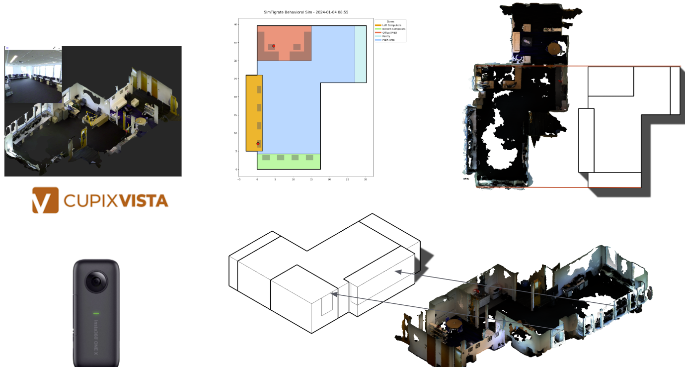
Figure: 3D capture and simplified zoning support the translation from whole-room occupancy to region-level occupancy information.
Synthetic Occupancy Data for Pipeline Testing
Because continuous real sensor data is still being integrated, the project uses behavior-informed synthetic occupancy data to test the pipeline. The fake data is not intended to replace real sensing. It is used to validate the data structure, zone-assignment logic, CSV outputs, and downstream simulation compatibility.
The synthetic schedule is designed to be more realistic than a fixed default schedule. It includes academic-calendar effects, semester variation, exam-period changes, summer reduction, holiday interruption, weekday patterns, and room-specific occupancy assumptions.
This allows the team to test whether whole-room counts can be converted into L1–L4 outputs, whether zone-level counts remain consistent with total room count, and whether people and equipment gains can be exported in a format usable by simulation tools.
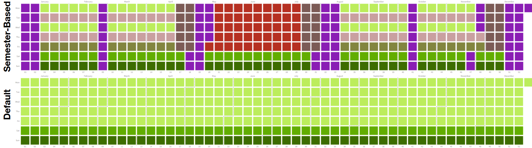
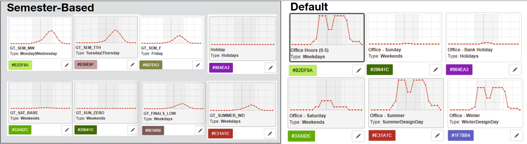
Figure: Semester-based synthetic occupancy data and spatial behavior logic used to test the pipeline before continuous sensor deployment.
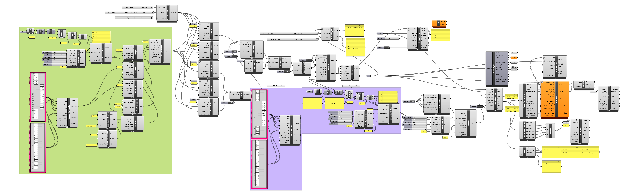
Data Processing Pipeline
Outputs & Configuration
- The pipeline writes a per-timestep CSV and an optional GIF visualization.
- Main CSV (
outputs/output.csv) includes: timestamp; L1 presence (hysteresis-smoothed); L2 whole-room count and occupancy fraction; L3 per-zone count and fraction; L4 per-zone people heat gain (W); L4 per-zone equipment state (devices on, W/m², total W); and room-level total internal gains. - Per-zone CSVs are written to
outputs/zones/<zone_name>.csv. - Time resolution and smoothing are controlled in
config.pyviaTIMESTEP(default5min),COUNT_SMOOTHING_WINDOW, andHYSTERESIS_WINDOW. - Toggle visualization with
ENABLE_VISUALIZATION; geometry and per-zone areas come from the physical map utilities.
GIF (optional)
- When
ENABLE_VISUALIZATION = True, one frame per timestep is rendered and assembled intooutputs/occupancy_sim.gif. - Each frame shows the floor plan with colored functional zones, furniture overlays, and red points for agent positions.
- Zone color key: Left Computers = orange, Bottom Computers = light green, Office = tomato, Pantry = light cyan, Main Area = sky blue.
Typical Runtimes
- Example: (10 nominal capacity, 5 zones,
TIMESTEP='5min') — simulation + CSV export for 10 days (LIMIT_HOURS = 240) runs in under 1 minute on a modern desktop. Frame rendering dominates cost when visualization is enabled.
Simulation Engine & Spatial Mapping
- Pipeline stages: ingest, process, export. Inputs are either a schedule CSV or a sensor CSV; both normalize to a
Human_Counttime series and a scenario label before processing. - Per-timestep processing: resample to
TIMESTEP, smooth viaCOUNT_SMOOTHING_WINDOW, clip to[0, NOMINAL_CAPACITY], and convert to integer counts. - For each timestep, agent positions are either sampled from the behavioral engine in
phys_map.pyor read from sensorPositions. Positions are assigned to zones and L3/L4 metrics are computed. Per-zone CSVs are exported.
Key Math & Logic
- Zone-sum hard constraint (L3): for every timestep \(t\),
$$ \sum_{z} n_z(t) = N(t) $$
where \(n_z(t)\) is the zone count and \(N(t)\) is the whole-room count.
- People heat gain (L4): fixed per-person assumption (145 W):
$$ Q_{\text{people}}(t) = 145 \times N(t) $$
Zone-level people gains use \(n_z(t)\) analogously.
- Equipment heat gain (L4): active device count per zone \(k_z(t)\) persists for
COMPUTER_AWAY_HOLD_STEPS. Equipment gain per zone:
$$ Q_{\text{equip},z}(t) = k_z(t) \times q_z $$
W/m² normalization used by building models is \(Q_{\text{equip},z}(t)/A_z\), where \(A_z\) is the zone area.
- Presence hysteresis (L1): presence is the rolling maximum over
HYSTERESIS_WINDOWsteps on the resampled counts to avoid rapid toggling:
$$ L1(t) = \mathbb{1}[\max_{t'\in[t-w,t]} N(t') > 0] $$
- Scenario inference: each day is labeled (
holiday,summer,finals,normal) based on mean/peak occupancy fractions; the chosen scenario alters agent behavior profiles.
Components
sim.py: ingests schedule or sensor CSVs, resamples and smooths counts, requests positions (behavioral or sensor), computes L1–L4 metrics, and writesoutputs/output.csvand per-zone CSVs.phys_map.py: defines room geometry (Shapely polygons), zone capacities, seat registry, and the behavioral agent engine that generates synthetic positions respecting zone capacities and scenario profiles. Agent persistence and departure logic are implemented here.visualization.py: renders zone polygons, furniture overlays, and agent positions to frames; frames are combined intooutputs/occupancy_sim.gif. Disable rendering withENABLE_VISUALIZATION = Falsefor CSV-only runs.
How to use the outputs
- The CSV outputs provide per-timestep L1–L4 signals suitable for downstream simulation tools (presence schedules, people and equipment internal gains, per-zone load densities).
- Visualization is optional and intended for debugging and presentation.
Hardware System
Hardware Overview
The hardware layer is responsible for collecting privacy-sensitive occupancy evidence before it is converted into L1–L4 simulation inputs. The system uses MLX90640 infrared thermal array cameras connected to ESP32 microcontrollers. Each MLX90640 returns a low-resolution grid of temperature values rather than a normal RGB image, allowing the project to detect human presence and approximate location without collecting identifiable visual information.
The hardware system currently supports the following sensing path:
thermal camera field of view
  -> 32 x 24 temperature matrix
  -> ESP32 data acquisition through I2C
  -> temperature frame storage / serial transfer
  -> MATLAB visualization and human-detection logic
  -> occupancy count and approximate position output
Sensing Device: MLX90640 Thermal Camera
The selected thermal sensor is the MLX90640 infrared array thermal imaging camera. It was chosen because it provides more spatial information than a single-point PIR sensor while still preserving occupant privacy better than a visual camera.
Key reasons for using the MLX90640 include:
- Privacy preservation: the sensor measures temperature values instead of capturing identifiable facial or visual images.
- Room-scale spatial information: the camera provides a 32 × 24 array, giving 768 temperature readings per frame.
- Wide field of view: the wide-angle version supports broad room coverage, making it suitable for ceiling or high-wall placement.
- Occupancy-relevant outputs: the thermal matrix can be processed into presence, approximate count, and approximate spatial location.
- Low-cost deployability: the sensor can be paired with ESP32 microcontrollers for a compact and relatively inexpensive prototype.
In the current detection approach, people are identified as warmer regions compared with the surrounding room background. The code scans the temperature matrix for clusters where the measured temperature is roughly 5 °C above ambient. These hot regions are grouped into blobs, and the system estimates a centroid or bounding region to approximate the occupant location.
Microcontroller Interface: ESP32
The MLX90640 cameras are connected to ESP32 microcontrollers, which handle sensor communication and data acquisition. The ESP32 interfaces with the cameras using the I2C communication protocol, allowing the microcontroller to request thermal frames from the sensors.
In the prototype workflow, the ESP32 collects thermal frames and formats the readings as temperature arrays. These arrays can then be sent to a computer for live visualization or stored locally for later processing.
Planned final hardware configuration:
- Two wall-powered ESP32 microcontrollers
- Two MLX90640 cameras connected to each ESP32
- 5 V wall adapters connected to the ESP32 5 V input pins
- SD card storage on the ESP32s for trial data collection
- Data accessed on demand instead of requiring a continuous live laptop connection
Using multiple ESP32s is important because placing all cameras on one microcontroller would require long wiring runs across the room. Long I2C wiring can introduce signal-integrity problems because added resistance, capacitance, and electrical noise can corrupt communication between the ESP32 and the cameras. Splitting the cameras across two ESP32s keeps wire lengths shorter and improves reliability.
Camera Installation and Room Coverage
The room-scale deployment uses four thermal cameras arranged across the room. Each camera captures one segment of the space, and the camera coverage regions are designed to overlap. These overlap zones help reduce blind spots and make cross-camera spatial mapping more robust.
The installation concept is:
- Mount cameras near the ceiling or upper room boundary to view the occupied floor area.
- Assign each camera to a portion of the room.
- Use overlap regions between camera fields of view to reduce missed detections.
- Combine individual camera frames into a fused room-level thermal snapshot.
- Map detected hot regions into room coordinates for occupancy count and approximate position.
This multi-camera layout supports the project goal of moving beyond simple occupied/unoccupied sensing. Instead of only detecting whether someone is present, the hardware can provide approximate spatial distribution, which is needed for L3 zoning and L4 activity/equipment proxy assumptions.
Data Collection and Human Detection
Each MLX90640 frame is treated as a temperature matrix. The current visualization and detection workflow is supported by a custom MATLAB program. MATLAB reads the thermal data, displays a heatmap, and prints estimated human count and approximate coordinates.
The basic detection logic is:
- Read the 32 × 24 thermal frame from the MLX90640.
- Estimate or define the ambient room temperature.
- Apply a threshold of about ambient + 5 °C to identify possible human regions.
- Group adjacent hot pixels into blobs.
- Filter small/noisy blobs that are unlikely to represent a person.
- Estimate occupant centroid or bounding box location.
- Export the number of detected humans and their approximate
(x, y)coordinates.
The output from this hardware layer can then be converted into the same structure used by the simulation pipeline: L1 presence, L2 count, L3 spatial distribution, and L4 activity/equipment proxy variables.
Current Prototype Status
The current prototype demonstrates the full sensing concept at a small scale: an MLX90640 camera connected to an ESP32 on a breadboard, with thermal frames visualized and processed externally. The final form factor will move toward a more deployable arrangement with wall-powered ESP32s, shorter camera wiring, and SD card-based data storage.
At this stage, the hardware system is intended to collect occupancy evidence for simulation and validation. It does not directly control HVAC equipment. Future work will focus on completing the four-camera installation, collecting real room data, validating detection accuracy, and replacing synthetic occupancy inputs with measured thermal-camera outputs.
Simulation Workflow
Grasshopper workflow outputs are organized around the same L0-L4 occupancy-information hierarchy used throughout the sensing pipeline.
Results / Visualizations
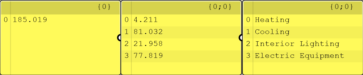
L0: Fixed Schedule Baseline
Occupancy: fully occupied at all times from 6am-7pm, Mon-Fri
Activity: all seated, 120W per person
Lighting: on at all times from 6am-7pm, Mon-Fri
Equipment: on at all times from 6am-7pm, Mon-Fri
Ventilation: constant value, 6am-7pm, Mon-Fri
Setpoint: heating 20℃, cooling 24℃
HVAC Availability: on at all times from 6am-7pm, Mon-Fri
Analysis Period: a whole year (applies to all levels)
L1: Presence-Based Occupancy
Occupancy: (fully) occupied/unoccupied
Activity: all seated, 120W per person
Lighting: on at all times from 6am-7pm, Mon-Fri
Equipment: on at all times from 6am-7pm, Mon-Fri
Ventilation: on/off according to occupancy
Setpoint: heating 20℃, cooling 24℃
HVAC Availability: on/off according to occupancy
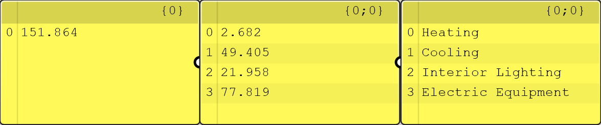
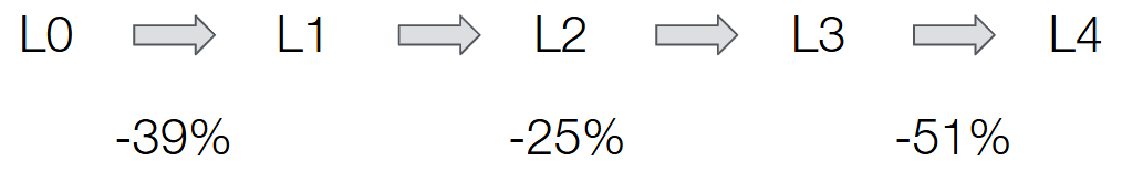
Heating energy use (2.682 kWh/m2) reduced by 36% compared to L0 (4.211)
Cooling energy use (49.405) reduced by 39% compared to L0 (81.032)
L2: Count-Based Occupancy
Occupancy: people count
Activity: all seated, 120W per person
Lighting: on at all times from 6am-7pm, Mon-Fri
Equipment: on at all times from 6am-7pm, Mon-Fri
Ventilation: air flow rate varies according to occupancy
Setpoint: heating 20℃, cooling 24℃
HVAC Availability: on/off according to occupancy
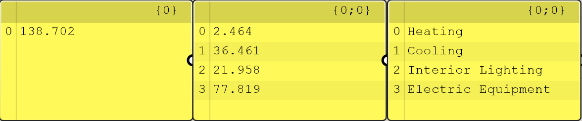
Heating energy use (2.464 kWh/m2) reduced by 8% compared to L1 (2.682)
Cooling energy use (36.461) reduced by 26% compared to L1 (49.405)
L3: Zoning
At this level, occupants are mapped to functional room zones before downstream simulation.
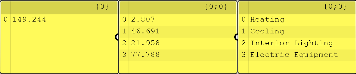
L4: Activity and Equipment Schedules
Occupancy: people count
Activity: varies
Lighting: on at all times from 6am-7pm, Mon-Fri
Equipment: on/off according to equipment schedule
Ventilation: air flow rate varies according to occupancy
Setpoint: heating 20℃, cooling 24℃
HVAC Availability: on/off according to occupancy
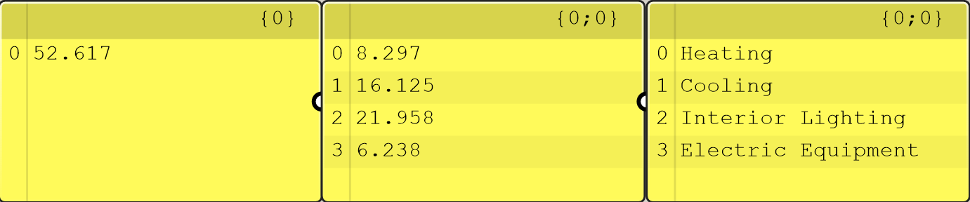
Turning off equipment helps reduce cooling energy use. Although there is an increase in heating energy use, total air conditioning load (24.422) is 51% less than L3 (49.498).
Discussion and Next Steps
The proportions of heating and cooling energy use does not seem reasonable. Admittedly, human generates heat, which causes more cooling load but compensates for heating, but it shouldn’t make such a huge a difference. A possible explanation is that the Honeybee engine overestimates the impact of heat generated by people. At the current stage, the comparison in heating/cooling among different levels is more valid than the comparison between heating and cooling at a certain level.
According to the results, the energy saving potential of HVAC control based on occupancy is obvious, but it seems too good to be true.
Possible cause:
- The base case is probably too rough, it is assumed at L0 that the room is always fully occupied from 6am-7pm, Monday to Friday. However, in common air conditioning load calculations of offices, the assumed occupancy may be 10% from 7am to 9am (considering workers who come early), 90% from 9am to 11am, 20% from 11am to 1pm (considering lunch break), 90% from 1pm to 5pm, 10% from 5pm to 7pm (considering workers who leave late). The long schedule and high occupancy of L0 makes energy use at this level to be very high, making energy use at other levels seem much lower in comparison.
- The equipment schedule doesn't correspond to the occupancy schedule at L1-3. At L1-3 it is assumed that the equipment is always on from 6am-7pm, Monday to Friday, and equipment also generates a lot of heat which needs to be addressed by cooling. However, the schedule of equipment often correspond to the schedule of occupancy in reality (the equipment will be turned off when the person leaves). If we assume that the equipment schedule corresponds to the occupancy schedule at L1-3, the energy use will drop further so that the gap in energy use to L4 will be smaller.
The current project should be understood as a prototype pipeline rather than a validated HVAC control system. The main contribution at this stage is the workflow structure: privacy-sensitive sensing or synthetic occupancy inputs can be translated into progressively richer HVAC-relevant simulation inputs.
Next steps include completing hardware deployment, collecting real thermal sensor data, validating presence/count/location detection, replacing synthetic inputs with measured sensor outputs, completing the baseline versus occupancy-informed simulation comparison, and adding formal metrics such as missed occupancy minutes, false-operation minutes, cycling count, energy use, and comfort indicators.
References
-
Clevenger, C. M., & Haymaker, J. (2006). The impact of the building occupant on energy modeling simulations.
Used to support the claim that occupant-related assumptions can strongly affect energy simulation outcomes. -
Kong, M., Dong, B., Zhang, R., & O’Neill, Z. (2022). HVAC energy savings, thermal comfort and air quality for occupant-centric control through a side-by-side experimental study. Applied Energy, 306, 117987.
Used to support the value of occupancy-based HVAC control for energy savings, comfort, and perceived IAQ. -
Yan, D., O’Brien, W., Hong, T., Feng, X., Gunay, H. B., Tahmasebi, F., & Mahdavi, A. (2015). Occupant behavior modeling for building performance simulation: Current state and future challenges. Energy and Buildings, 107, 264–278.
Used to support the need to monitor, model, evaluate, and implement occupant behavior in building simulation workflows. -
Chen, Z., Jiang, C., & Xie, L. (2018). Building occupancy estimation and detection: A review. Energy and Buildings, 169, 260–270.
Used to support the comparison of occupancy sensing methods, including PIR, cameras, CO₂, and sensor fusion. -
Esrafilian-Najafabadi, M., & Haghighat, F. (2021). Occupancy-based HVAC control systems in buildings: A state-of-the-art review. Building and Environment, 197, 107810.
Used to support the link between occupancy detection, occupancy prediction, and HVAC control strategies. -
D’Oca, S., & Hong, T. (2015). Occupancy schedules learning process through a data mining framework. Energy and Buildings, 88, 395–408.
Used to support the idea that occupancy schedules can be learned from data rather than assumed from fixed standards. -
Lou, Y., Ye, Y., Zuo, W., & Zhang, J. (2021). Energy prediction impact of the space level occupancy schedule for a primary school. Proceedings of Building Simulation 2021.
Used to support the distinction between building-level and space-level occupancy schedules in energy modeling.
Presentation